notes on lineage inpainting
an informal companion to the paper
A goal of developmental biology is to model the process by which cells acquire their fates. Single-cell sequencing reveals the states cells occupy but not the dynamics that connect them, because each cell can be profiled only once. Recent methods model these dynamics from static snapshots, typically aiming to predict a cell's past and future from its present molecular state. Yet it is thought that measured transcriptional states are not fully informative about dynamics: cells in similar transcriptional states can arise from different origins or be biased toward different fates. Here we explore the possibility that additional information about dynamics can be recovered from a cell's lineal context (sisters, cousins, and so on). We introduce lineage inpainting, a generative modeling approach that operates over entire lineage trees rather than reconstructing individual cell trajectories.
This little website gives an informal introduction to the methods we use and tries to build intuition for why we use them and what they can help us learn. There will be some fun pictures and at least one interactive vis along the way :)
a model of development
some motivating inuitition
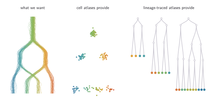
We want a model of development. What exactly does this mean? We'll be more precise about it later. But loosely, we want to take an embryo (defined by a population of cells and the states they occupy), and play the tape forward/backward through cell division and differentiation, to see an embryo at a later/earlier timepoint. In other words, we'd like a (probabilistic) movie of mouse development.
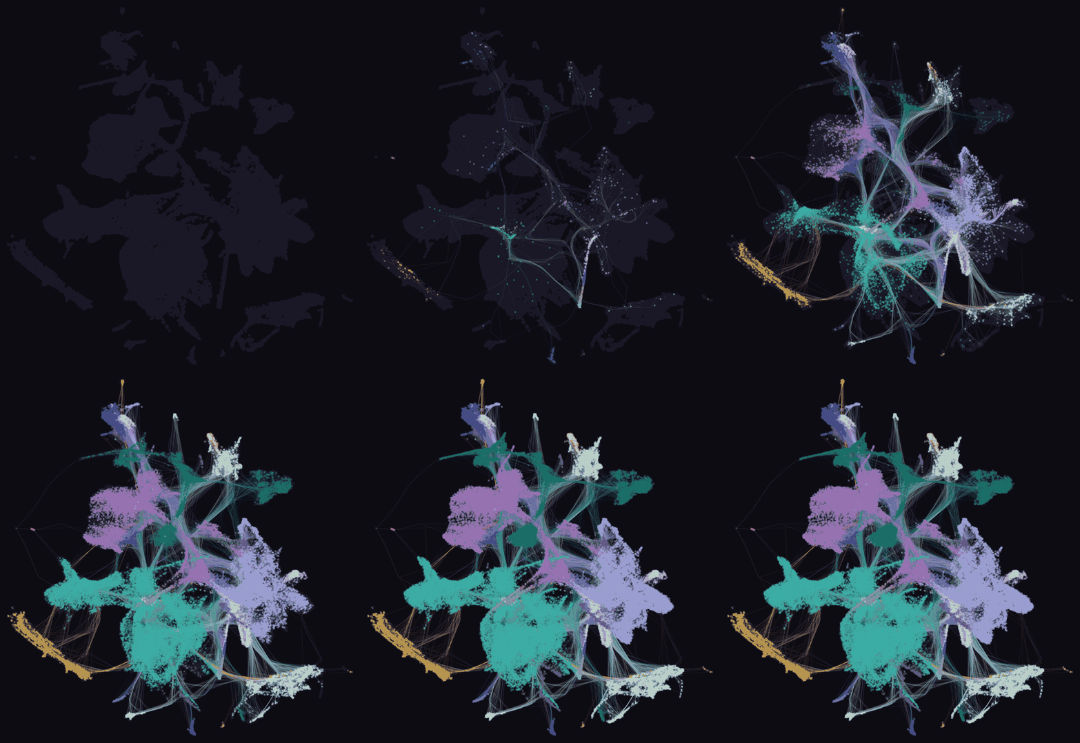
In the past decade or so, there has been a huge proliferation of single cell atlases, which use techniques like single cell RNA sequencing (scRNA-seq) to profile the molecular states of cells across embryos at different times. These atlases have been extremely informative, but do not directly tell us anything about dynamics (that is, how cells transition between states) because scRNA-seq is destructive, and results only in snapshots. The same cell can't be profiled twice.
In response to this limitation, a great amount of work has gone into trying to model dynamics from snapshot measurements alone. A number of generative modelling approaches, building on optimal transport, neural ODEs/SDEs, and flow matching have been explored for the cell state dynamics problem. These methods typically take as input a single cell's transcriptomic profile, and predict the past or future of a cell using its current molecular state alone. That is, they are Markovian with respect to transcriptomic states.
However, a cell's measured transcriptional state is not fully informative about where it is going. This has been shown formally in hematopoiesis by work from Allon Klein's group. It also aligns with (I think) most people's biological intuitions. Things like methylation states are not visible transcriptionally but do influence dynamics, and there is a recent paper where drosophila intestinal stem cells appear to make fate decisions based on a cell division counter (switching fates every 8 divisions).
Here we explore the possibility that information about dynamics can be extracted from a cell's lineage context, as measured by lineage-traced scRNA-seq. We introduce a computational approach we call lineage inpainting, a generative model of dynamics which operates over an entire tree simultaneously rather than one cell at a time. To do this, we develop a tree-structured attention mechanism.
lineage-traced scRNA-seq
what our data looks like
Single-cell RNA sequencing (scRNA-seq) tells us, for each measured cell, how strongly expressed each gene is. The data is typically preprocessed into count vectors where each entry represents the abundance of a particular gene. This gene expression vector can be thought of as a cell's state in a high dimensional space.
Each cell can be sequenced only one time. So we can never get a time-series of the expression of a single cell. But what we can get are population-level snapshots of different populations at different times. And from these population level snapshots, one can try to reconstruct the trajectories of individual cells. This is often called trajectory inference or dynamic inference, and numerous methods have been developed to do this. Many build on the mathematical framework of optimal transport. (what we mentioned briefly in the previous section)
But the problem is fundamentally underconstrained. Infinitely many movies can give rise to the same set of snapshots. In order to break this degeneracy, you have to make some assumptions, and these assumptions may not always match what happens in biology. Optimal transport methods, for instance, typically assume that cells move minimally in gene expression space.
lineage tracing
Recent lineage tracing techniques can give us extra information to constrain these dynamics. While lineage tracing is quite a broad term, here we are referring to experimental methods which are able to tell us how closely related any pair of cells are: that is, are they sisters, first cousins, and so on. From these pairwise measurements, many methods exist to reconstruct cell lineage trees.
These lineage trees tell us something about dynamics, but fundamentally they are still snapshot measurements. We do not see the cell states at internal nodes on the tree.
warning! a common misunderstanding
People often assume that we get to see the states at the internal nodes of the tree. This is not true in our settings.
what about the lineage tracing datasets where the same clones are observed twice?
In some lineage-traced scRNA-seq datasets of cells cultured in a dish, it is sometimes possible to measure the same tree at two different depths. But it is never possible to measure the same trajectory twice by scRNA-seq, and it is never possible to measure the same tree at two different depths when working with whole organisms. In a dish, you can take half the cells and allow the rest to continue to proliferate. This is not possible, at least not to my knowledge, in a mouse.
So a cell lineage tree provides strong constraints on dynamics, but don't fully specify them. The tree tells us who is related to whom, and the leaves tell us where they ended up. But we observe nothing about the states at the internal nodes of the tree, and as such we have no explicit information about dynamics.
generative models of developmental trees
making the problem precise
Before building our lineage inpainting machinery, we'll say more formally what we mean by a generative model of developmental trees.
We define a lineage tree as a set of nodes $V$ with edges $E$ and node times $\tau$, and each node $v$ carries a state $x_v$. Some states are hidden, $x_M = \{x_v : v \in M\}$ of a subset of nodes $M \subset V$ the goal of the model is to sample them conditional on everything that remains: the topology, the node times, the visible states, and which nodes were hidden. Writing this context as
$$ \mathcal{C} = (V, E, \tau, \{x_v : v \notin M\}, M), $$
the goal is to model $p(x_M \mid \mathcal{C})$.
Depending on which nodes are hidden, different questions can be asked. If the leaves are observed and the internal nodes are hidden (part of $M\in V$), then this is sampling from the ancestral state distribution. If an internal layer has observed states but the nodes below are unobserved in $M$, then this is descendant inference.
Throughout, we take the tree topology and the node times as given, and model only the states on the tree. This is a practical choice. We also show that it is possible to regress descendant number on state in a reasonable way, if one also needed at test time to generate tree topologies (though in practice we have ways to work around this for most tasks we're interested in).
impute and sample
a framework for fitting generative models to (incomplete) trees
Before considering modeling dynamics on the tree, we'll first briefly introduce some existing approaches to modeling dynamics without the tree.
A number of recent methods (including GENOT and OT-CFM) model dynamics between a pair of cell populations by first computing an optimal transport coupling (cell-cell correspondences between cell populations) and then fit a flow matching model to match the empirical OT coupling.
We can think about this process abstractly as imputing (choosing a coupling between cells at different times) and sampling (fitting a generative model which will match the imputed dynamics).
The same recipe can apply to learning dynamics on trees. We can think about imputing as filling in the internal nodes using some recipe, and sampling as fitting a generative model to match the trees with imputed states. And I think any strategy for fitting a generative model on lineage trees can be thought about in this way.
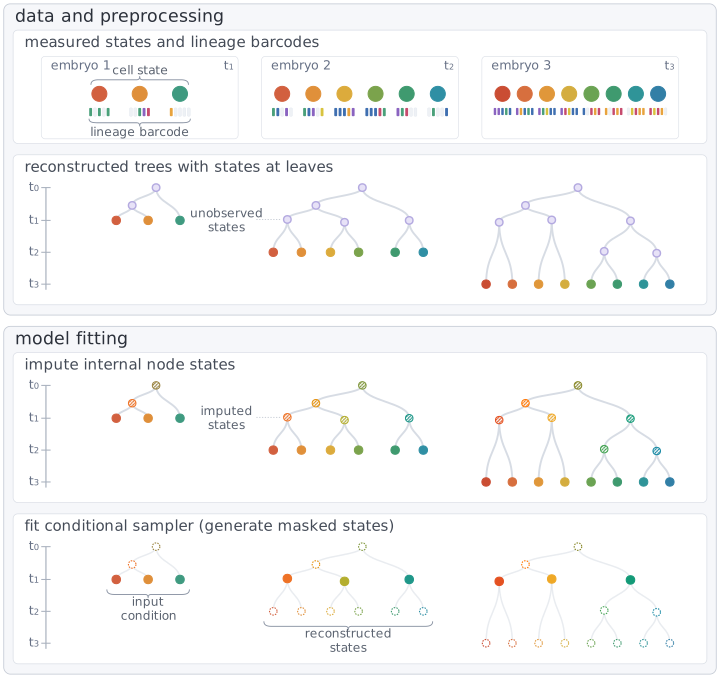
What we will introduce next is an imputation method (which itself learns a coupling, rather than imposing an optimal transport coupling), a sampling method which generates entire trees simultaneously, and a tree-structured transformer architecture which underlies both.
learning an imputation model
from phylogenetics to cell lineages
The problem of imputing ancestral states on the tree, filling in the internal nodes, is analogous to an old problem in phylogenetics. There, one observes some traits of extant species (like tail lengths of all living lizard species) and tries to infer the traits of ancestral species (like the tail length of an extinct lizard).
This is similar to our setting, with one major difference. In phylogenetics you only get to see one tree, at one time -- you cannot get multiple samples of evolution at different times. In lineage-traced scRNA-seq, however, we can measure different organisms, measured at different timepoints.
felsenstein's method
The simplest approach is to ancestral state inference, proposed long ago by Felsenstein, is to infer a parent's state as the mean of a children. Each internal node state becomes
$$ \hat{x}_v = \frac{1}{|\mathrm{ch}(v)|} \sum_{u \in \mathrm{ch}(v)} \hat{x}_u, $$
evaluated recursively up from the leaves, so that by the time a node is reached both of its children already have values. If you assume the dynamics are Brownian, this $\hat{x}_v$ is the posterior mean.
This ancestral state inference method is totally parameter-free, and actually works quite well in many cases. For example, if all your descendants are in the same state, it's not unreasonable that you also will be in the same state.
why our imputation problem is "easier"
A recursive mean is a sensible thing to do if you only have one timepoint (one tree, with states only at the leaves). But unlike the phylogenetics setting, we actually have a lot more information about what the ancestral states should look like. So we can hope to learn a more complicated ancestral inference function rather than just this recursive mean.
We do not know what each individual node should be, but we know what the tree should look like at an earlier timepoint, based on the actual measured trees at those earlier timepoints. So we can enforce that an imputed tree should match actually measured trees at different timepoints. In the next section, we'll make more precise how we can optimize for this kind of consistency.
the alignment loss
how to tell if two trees are the same
Learning an ancestral inference function is not straightforward, because we never actually observe the exact ancestral state. We observe an ancestral population, but never the precise ancestor of a set of cells. So we can't simply regress using a node-wise error. But instead, we can evaluate imputations at the distributional/population/tree-level.
Imputing the ancestors of a tree captured late in development yields a prediction for the populations at earlier timepoints, and we can compare these against true measurements of other embryos at earlier timepoints. A good ancestral reconstruction will match the distribution of the states at each time from the trees we observed at each of those times. Because each tree anchors this comparison to real data at a different time, requiring all trees to agree constrains the inferred dynamics to be consistent with our snapshot observations.
We make this precise with an alignment loss that minimizes the distributional distance, across trees, between what we call tree features. The simplest and most essential tree feature is the state of a single cell and its corresponding time. Matching the distribution of these across trees makes the cell population at each time point consistent from one tree to the next.
This alone is not sufficient, because a model can reproduce the correct distribution of states at every time while still completely distorting the tree structure. So we also align higher-order tree features, including pairs of sister-cell states and trajectories of states across time. Our alignment loss is the sum of the distributional distance of several tree features, between each pair of trees.
the alignment loss in practice
The two features we look at, in addition to the cell state feature which matches the time marginals, are what we call the path feature and the common ancestor feature.
The path feature means that between trees, individual trajectories, paths through the Waddington landscape if you will, should match. The cousin feature says that pairs of $\alpha$-cousins which share a common ancestor at time $t - \alpha$ should match between trees.
We can think of the path feature as matching "tall" dependence structure on the tree, and the common ancestor feature as matching "wide" dependence structure.
In the theory supplement, we show that these features are a practical restriction of a more general metric between lineage trees.
features we implement and how they are defined in the codebase:
| feature | what it compares |
|---|---|
TimeMarginalFeature |
states in a time slice |
PathFeature |
root-to-leaf trajectories on a common grid |
CommonAncestorFeature |
states of a triplet of two cells sharing a common ancestor at time and their ancestor |
So given a neural network architecture that can impute ancestors on a tree, we can use this alignment loss to ensure the imputations are consistent. But what architecture should we use?
a tree-structured transformer
an architecture for lineage trees
As we mentioned in the intro, a cell's fate and history are not fully determined by its current transcriptional state alone. Cells sharing a recent ancestor inherit common factors that indicate their origin and shape how they develop. A single-cell level predictor is not able to leverage this shared information. So something like an MLP which predicts ancestor/descendant from current state is not ideal, at least in theory.
Instead, we would ideally like a model that can process an entire tree, each cell alongside all of its relatives, at once. Here we show how a simple extension of the transformer architecture allows us to do this.
The transformer is the architecture at the heart of modern language modeling, but it is actually a general purpose tool for processing sets of tokens. In language each token is a few characters in a sentence, and the transformer uses a mechanism called attention to allow each token to aggregate information from all others. Here, instead, each token represents a cell state. Learned projections map token $i$ to a query $q_i$, key $k_i$, and value $v_i$, and attention updates it by averaging the values according to how well its query matches each key:
$$ h_i = \sum_j \alpha_{ij} v_j, \qquad \alpha_{ij} \propto \exp\left(\frac{q_i^\top k_j}{\sqrt{d_k}}\right), $$
with $\alpha_{ij}$ normalized over $j$ and $d_k$ the query and key dimension. The update therefore combines information from the cells assigned the largest weights.
encoding tree structure in the attention mechanism
On its own, attention treats its inputs as an unordered set, so the cells in the tree can only depend on each other through their states, not on how they are related. Transformers for language conventionally repair this with positional encodings, embeddings of each token's position added to its input. But these presume a 1D sequential ordering, like a token's position in a sentence, which cells across a branching tree do not have.
An alternative approach is to encode relative position information in the attention mechanism by adding distance-dependent biases to the attention logits (this is used by ALiBi for 1D sequential data). This generalizes to any setting where we have a pairwise distance between tokens, and we have a natural distance between cells on a lineage tree.
We use the patristic distance $\operatorname{pat}(i,j)$ between two cells: the total branch length along the path joining them through their most recent common ancestor. We add it to each pair's attention logit before normalization, scaled by a learnable weight $\gamma^{(l,h)}$, one per layer $l$ and head $h$:
$$ \alpha_{ij} \propto \exp\!\left(\frac{q_i^\top k_j}{\sqrt{d_k}} + \gamma^{(l,h)}\,\operatorname{pat}(i,j)\right) $$
In practice $\gamma^{(l,h)}$ comes out negative across layers and heads, concentrating attention on closer relatives. You can see how the tree-structure bias works in the interactive visualization below.
b-sides: tree encodings that did not make the cut
We spent a long time thinking about how to get a tree-structure into the architecture. A really fun idea that Nic came up with was to simulate a branching stochastic process with the same topology as the lineage tree, then add the (random) value of the process to the token at the corresponding node of the tree. Very cute -- but ended up not being as robust as the attention bias.
imputing with the transformer
how the architecture actually fills in the tree
So we have an architecture that reads a whole tree, and a loss that says whether an imputation is good. Next we'll show how to combine them to learn an imputer.
As input, we begin with a subtree where the states at the leaves were observed, and the internal node states are to be imputed. Each node gets a corresponding token. For the observed leaves, the token is the state. For the unobserved internal nodes, the states are random samples of a Gaussian. We pass this through the tree-structured transformer, and as the output, we get a vector for each node. These vectors are not directly the predicted states, but can be used to find the predicted states through some arithmetic (this will make sense shortly).
predicting the Felsenstein residual, rather than the state directly
The network does not predict a node's state outright. Each masked node first gets a baseline. For nodes above the anchors (nodes with observed states), the baseline is the recursive mean of its children, which is exactly Felsenstein's method from earlier. For nodes below the anchors, it is the nearest anchor's state carried down. The transformer then predicts the difference between the true state and that baseline, and the baseline is added back.
So the model starts from a Felsenstein baseline and learns a correction to it. This choice matters a lot in practice: predicting the residual rather than the state improves things dramatically.
applying the loss
We can take two trees at different times, then apply the imputer to get predicted internal node states for many subtrees from each "big" tree, then use the alignment loss to see how distributionally consistent the trees are.
snapping to real cells
The imputer produces cell state vectors as its predictions for internal nodes. But if the model is not perfect (which is very likely, as it is a one-step model trained with a population-level distributional loss), it can make predictions that are far from the data manifold. If we want the most realistic possible imputations, something we can do is "snap" the predictions to their nearest neighbors among the observed cells. Since we're working with an atlas of ~4M cells, I think it's safe to assume that most real states have been observed somewhere in our dataset. This choice will turn out to be later on, as we'll be training another model on the outputs of the imputer (and snapping to real helps prevent a collapse).
fitting a sampler
a tree-structured stochastic interpolant transformer
The imputer fills in the internal nodes of a tree (reverse in time). But it does not allow us to forecast descendants (forward in time), and nor does it allow us to test time scale, since it is only one step (that is, it often makes "fuzzy" predictions for cell states). So we now fit a more powerful sampler.
We want a generative model that takes a tree observed at a single generation and can sample the states of the ancestors that came before and the descendants that follow. To fit such a model, we take the complete trees produced by the imputation step and learn to inpaint states that we mask out, building on diffusion, flow, and stochastic interpolant based generative modeling techniques which have seen great success in computer vision.
Recall the context $\mathcal{C}$ from earlier: the topology, the node times, the visible states, and which nodes were hidden. We model $p(x_M \mid \mathcal{C})$ with a transformer $S_\phi$ that takes as input one token per node, both masked and unmasked. A visible node's token carries its state $x_v$. A hidden node's token instead carries an interpolant between noise and its true state,
$$ I_v(s) = \alpha_s\, x_v + \sigma_s\, x_1^v, \qquad x_1^v \sim \mathcal{N}(0, \mathbf{I}), $$
which is the true state at $s = 0$ and pure noise at $s = 1$, with $\alpha_s$ and $\sigma_s$ a variance-preserving schedule. We draw the noise independently at each hidden node, sample one interpolation time $s \sim \mathcal{U}[0,1]$ for the whole tree, and add an embedding of $s$ to every token. Each token also carries an embedding of its node time $\tau_v$.
At each hidden node $S_\phi$ predicts the clean state directly, and we minimize the squared error
$$ \mathcal{L}(\phi) = \mathbb{E} \sum_{v \in M} \| S_\phi(s, I, \mathcal{C})_v - x_v \|^2, $$
where $I$ collects the interpolants at the hidden nodes, and the expectation runs over a masked tree from our imputed data, the interpolation time $s$, and the noise. To sample, we set the hidden nodes to noise at $s = 1$ and integrate down to $s = 0$, using the prediction of $S_\phi$ to step the interpolant toward data.
The one thing to keep straight is that there are two times here and they have nothing to do with each other. $\tau$ is developmental time, running along the tree. $s$ is bridge time, running from noise to data. The bridge operates on an entire subtree at once, spanning node times across development.
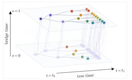
This can be thought of as a tree analog of stochastic interpolant methods for image inpainting and for imputing missing values in time series.
implementation tricks
details that turn out to matter
A few things turned out to matter more than expected. Each of these is an ablation, and the numbers behind them go in the results.
- it has to be end to end. we optimize the imputer and the sampler simultaneously. a surprising finding (to me at least) was that a stop grad between the imputer and the sampler kills performance. the imputer really benefits from gradients provided by the sampler.
- snap to real is good, but you have to alternate id-nn. explaining this is going to be unpleasant
- felsenstein initialization is important. we have the transformer architectures predict the residual from the felsenstein imputation, rather than the direct state itself. modeling the residual rather than the state actually dramatically improves performance.
one training step
Now we've introduced all the lineage inpainting machinery, and we can walk through what training looks like.
- sample two trees $r_1, r_2$ and a root time $t < \min(t_{r_1}, t_{r_2})$ (e.g. an E9 and an E9.5 embryo, $t = 8.5$)
- for each tree $r$:
- draw
n_subtreesnodes $u_1 \dots u_n$ with $\tau_{u_k} \approx t$, and take $\mathcal{T}^r_k$ to be the subtree under $u_k$ down to the observed leaves - for all internal nodes, impute: $\hat{x}^r_k = P_{\theta} (\mathcal C)$, a state at every node (Felsenstein baseline plus predicted residual)
- score the alignment loss between the two records' imputed subtrees, $\mathcal{L}_{\text{align}} = \sum_f d_f(\hat{x}^{r_1}, \hat{x}^{r_2})$, summing over tree features $f$ (marginal, path, common ancestor)
- (on alternating steps) snap: replace each imputed $\hat{x}_v$ by its nearest observed cell in the atlas
- for each subtree:
- sample an antichain $A$ (one "layer" cutting across the subtree) as anchors. mask everything else, $M = V \setminus A$, both above and below
- draw one $s \sim \mathcal{U}[0,1]$ and source noise samples, and form the interpolants $I_v(s)$ at the hidden nodes
- $\mathcal{L}_{\text{sample}} = \sum_{v \in M} \| S_\phi(s, I, \mathcal{C})_v - \hat{x}_v \|^2$
- $\theta, \phi \leftarrow$ optimizer step on $\lambda_{\text{align}} \mathcal{L}_{\text{align}} + \lambda_{\text{sample}} \mathcal{L}_{\text{sample}}$
code: one step of the trainer
synthetic data
recovering dynamics when we know the ground truth
in principle, lineage inpainting enables us to (1) learn dynamics which are "non-optimal-transport" or "non-least-action" and (2) learn dynamics that are context dependent (i.e. not predictable from current state alone).
we have some synthetic experiments that show this.
then we could explain the random cell type motif setups (or just defer this to the paper)
the mouse embryo
to be written
to be written
how does development go wrong?
repurposing an observational model to make counterfactual predictions
to be written